隐藏图片

如何用 100 行代码得到一个 Fillippov 系统的求解器

Fillippov 是一类分段光滑的 ODE (Ordinary Differential Equation) 系统, 该系统在相空间中存在着一个超曲面, 这个超曲面将矢量场分成两个部分, 这两个部分的矢量场是不同的. Fillippov 系统在一定条件下允许系统的轨线穿过这个超曲面, 甚至允许轨线在这个超曲面上滑移. 这样高度复杂的非光滑给数值计算带来了挑战. 然而凭借 Julia 中的 DifferentialEquation.jl 强大的事件处理能力, 我们将仅用 100 行代码实现这类 Fillippov 系统的求解, 并且该求解器是一般的, 适用于任意维度的 Fillippov 系统.

Fillippov 系统的基本性质

考虑 $\mathbb{R}^n$ 中的矢量场:

F(x)=\begin{cases}F_{1}(x),H(x)<0,\\F_{2}(x),H(x)>0,\end{cases}

其中 $F_1,F_2$ 均是 $\mathbb{R}^n$ 中的光滑矢量场, $H$ 是 $\mathbb{R}^n$ 中的光滑函数. 我们假设 $H(x)=0$ (我们将使用相应的等式或不等式表示满足该等式或不等式的点集的集合) 是空间中的一个超曲面. 我们假设区域 $\Omega_1,\Omega_2$ 分别是 $H(x)<0$ 与 $H(x)>0$ 对应的区域.

假设一条从 $\Omega_1$ 出发的以 $F_1$ 为矢量场的轨线到达了 $H(x)=0$ , 那么轨线应该如何继续前进呢? Fillipov 系统这样决定轨线的走向:

如果在到达点, 两边的矢量场均指向曲面 $H(x)=0$ , 那么轨线在曲面上滑行;
如果在到达点, 两边的矢量场有着顺流的趋势, 那么轨线穿过曲面, 在 $\Omega_2$ 以 $F_2$ 为矢量场继续运动
如果初始点选在曲面上, 两边的矢量场在曲面上均有离开曲面的趋势, 那么该点的解无定义.

上述方式确定了轨线曲面的附近该如何运动. 然而我们有两个问题:

如何数学上严格描述上述几种情况?
如果轨线在曲面上运动, 怎么定义在曲面上的矢量场?

下面我们参考文献 (Dieci (2011)) 给出上面两个问题的回答.

对于 $x\in H(x)=0$ , 令 $\nabla H(x)$ 为梯度矢量. 由假设 $F_1(x)$ 在 $H(x)<0$ 这一侧, 那么 $\nabla H(x)$ 指向 $\Omega_2$ 这一侧. 那么:

两边矢量场都指向 $H(x)=0$ 即:

\nabla H(x)\cdot F_1(x)>0\ \text{且}\ \nabla H(x)\cdot F_2(x)<0.

具有顺流的趋势:

(\nabla H(x)\cdot F_1(x))\times(\nabla H(x)\cdot F_2(x))>0.

两边矢量场都有离开 $H(x)=0$ 的趋势:

\nabla H(x)\cdot F_1(x)<0\ \text{且}\ \nabla H(x)\cdot F_2(x)>0.

下图解释了上述数学定义:

椭圆台球的轨迹

现在我们已经解决了第一个问题, 下面我们来看第二个问题. 我们这样定义在 $H(x)=0$ 处的矢量场, 令

\alpha(x)=\frac{\nabla H^T(x)F_1(x)}{\nabla H^T(x)(F_1(x)-F_2(x))}.

在 $H(x)=0$ 上的矢量场就定义为:

F_H(x)=(1-\alpha(x))F_1(x)+\alpha(x)F_2(x).

不难验证, 我们有:

\nabla H(x)\cdot F_H(x)=0.

程序求解思路

下面我们来介绍如何用程序实现求解 Fillippov 系统. 首先假设轨线从相空间中任一点出发, 根据系统特性, 我们将其分为两种可能, 第一种是在 $H(x)=0$ 上, 一种是不在 $H(x)=0$ 上.

我们首先来考虑后者, 那么我们可以照常积分轨迹, 但是要时刻监测解是否到达了分界面, 因此需要设置一个事件, 这个事件即 $H(x)=0$ 触发的事件. 假设解到了分界面, 首先其不可能是排斥的情况, 因此我们只需要判断解是穿越分界面还是在分界面上滑动. 这可以由我们之前介绍的条件来判定. 如果穿越了, 则切换到另外一边的矢量场, 并仍重复这之前的步骤; 如果在分界面上滑动, 那么我们需要立即切换到分解面上的矢量场. 但此时, 我们的解时刻满足 $H(x)=0$ , 因此我们必须要弃用之前的事件. 我们必须要采用一个新的事件, 这个事件可以判断解什么时候可以从分界面滑移出去. 停留在分界面上的条件是 (2), 那么由于解连续地变化, $H,F_1,F_2$ 也是光滑的, 那么如果不满足条件 (2) 中的不等式, 其一定是首先穿过了零. 那么我们就把

(\nabla H(x)\cdot F_1(x))\times(\nabla H(x)\cdot F_2(x))=0

当作我们在分界面上的事件. 如果这个零点条件满足, 我们接下来需要确定解是流向哪个区域, 这自然很简单, 如果:

\nabla H(x)\cdot F_1(x)<0

即表示解流向 $\Omega_1$ ; 如果:

\nabla H(x)\cdot F_2(x)>0

即表示解流向 $\Omega_2$ . 解离开分解面以后, 再重复之前的步骤直至达到积分终点即可.

代码实现及例子

上一节所叙述的求解思路有一定的复杂性, 我们需要让求解器进行许多判定, 主要的判定有两个, 第一个是我们要让求解器知道解是在滑动还是在正常的状态, 第二个求解器解需要判定事件发生时应该怎么处理, 是进入滑动状态还是离出滑动状态.

第二个判定我们可以用 DifferentialEquation.jl 中的事件处理来实现, 实际上许多微分方程的求解系统均对事件处理有接口, 我比较熟悉的是 Mathematica 中的 NDSolve 中的 WhenEvent 选项, 其可以定位事件, 并修改在事件发生时的解的状态, 或停止积分等. 第一个判定, 我们可以这样处理. 定义一个类:

struct ODESol
    solution # ODE solution solved by OrdinaryDiffEq.jl
    state::Symbol # only two symbols are used: :regularmode and :slidemode
end

这个类中有两个值, 第一个是默认求解器在某个矢量场, 即 $F_1,F_2,H_F$ , 求解出来的解, 第二个是这个解的状态. 我们使用两个状态就足够了: :regularmode 与 :slidemode, 分别表示解是在通常状态还是在滑动. 注意到, 一个解的最后一个时刻要么是最终的积分时间, 要么就是因为我们所定义的事件在这一时刻停止了积分. 这样我们通过读取该解的状态, 就可以知道解是不是在滑动, 并可以通过解的最后的状态来判定下个解应该在哪个区域求解, 它的状态是什么.

我们将上面的思路整理成下面的求解器 fillippov_solve, 由于我们已经将思路叙述清楚, 并在下面的代码中给出了详细的注释, 下面就不再逐行解读代码.

using StaticArrays, OrdinaryDiffEq, Plots, LinearAlgebra

struct ODESol
    solution # ODE solution solved by OrdinaryDiffEq.jl
    state::Symbol # only two symbols are used: :regularmode and :slidemode
end

function fillippov_solve(f1, f2, h, ∇h, v0, p0, t0, tend)
    # it is assumed that f1 is at h(x)<0 and f2 is at h(x)>0
    # f1, f2, h, ∇h are all type of f(u, p, t), the output is a vector
    # initial condition: v0 
    # time interval: t0,tend
    # parameter p0
    # 
    # first define the vector field on the switch surface
    function sv(x, p, t)
        α = dot(∇h(x, p, t), f1(x, p, t)) / dot(∇h(x, p, t), f1(x, p, t) - f2(x, p, t))
        (1 - α) * f1(x, p, t) + α * f2(x, p, t)
    end

    # the hyper surface 
    function newh(x, t, integrator)
        h(x, integrator.p, t)
    end
    # stop the integrator
    function stop(integrator)
        if (integrator.t-integrator.sol.t[1])< 1e-2 # to avoid the 
            nothing
        else
            terminate!(integrator)
        end
    end

    # exit the sliding mode when slide_exit=0
    function slide_exit(x, t, integrator)
        dot(∇h(x, integrator.p, t), f2(x, integrator.p, t)) * dot(∇h(x, integrator.p, t), f1(x, integrator.p, t))
    end

    # main data consist of different solutions at h>0, h<0 and h=0
    sols = Vector{ODESol}(undef, 1)

    if abs(h(v0, p0, t0)) < 1e-10 # if this happen, we assume that the initial condition is on h=0
        prob = ODEProblem(sv, v0, (t0, tend), p0)
        cb = ContinuousCallback(slide_exit, stop)
        firstsol = ODESol(solve(prob, Vern6(), callback=cb), :slidemode)
        sols[1] = firstsol
    elseif h(v0, p0, t0) > 0
        prob = ODEProblem(f2, v0, (t0, tend), p0)
        cb = ContinuousCallback(newh, stop)
        firstsol = ODESol(solve(prob, Vern6(), callback=cb), :regularmode)
        sols[1] = firstsol
    else
        prob = ODEProblem(f1, v0, (t0, tend), p0)
        cb = ContinuousCallback(newh, stop)
        firstsol = ODESol(solve(prob, Vern6(), callback=cb), :regularmode)
        sols[1] = firstsol
    end
    while sols[end].solution.t[end] != tend # if the last of sols's time ≠ tend
        v1 = sols[end].solution.u[end]
        t1 = sols[end].solution.t[end]
        if sols[end].state == :slidemode # if the last solution is in slidemode, we have to determine which vector field it enter
            if abs(dot(∇h(v1, p0, t1), f2(v1, p0, t1))) < 1e-8 && dot(∇h(v1, p0, t1), f1(v1, p0, t1)) > 1e-5
                prob = ODEProblem(f2, v1, (t1, tend), p0)
                cb = ContinuousCallback(newh, stop, repeat_nudge=0.2)
                firstsol = ODESol(solve(prob, Vern6(), callback=cb), :regularmode)
                append!(sols, [firstsol])
            elseif abs(dot(∇h(v1, p0, t1), f1(v1, p0, t1))) < 1e-8 && dot(∇h(v1, p0, t1), f2(v1, p0, t1)) < -1e-5
                prob = ODEProblem(f1, v1, (t1, tend), p0)
                cb = ContinuousCallback(newh, stop, repeat_nudge=0.2)
                firstsol = ODESol(solve(prob, Vern6(), callback=cb), :regularmode)
                append!(sols, [firstsol])
            else
                break
                print("The solution is not defined on state $v1 and time $t1")
            end
        else
            if dot(∇h(v1, p0, t1), f1(v1, p0, t1)) * dot(∇h(v1, p0, t1), f2(v1, p0, t1)) > 0 # crossing h=0
                if dot(∇h(v1, p0, t1), f1(v1, p0, t1)) > 0
                    prob = ODEProblem(f2, v1, (t1, tend), p0)
                    cb = ContinuousCallback(newh, stop, repeat_nudge=0.2)
                    firstsol = ODESol(solve(prob, Vern6(), callback=cb), :regularmode)
                    append!(sols, [firstsol])
                else
                    prob = ODEProblem(f1, v1, (t1, tend), p0)
                    cb = ContinuousCallback(newh, stop, repeat_nudge=0.2)
                    firstsol = ODESol(solve(prob, Vern6(), callback=cb), :regularmode)
                    append!(sols, [firstsol])
                end
            else # entering h=0
                prob = ODEProblem(sv, v1, (t1, tend), p0)
                cb = ContinuousCallback(slide_exit, stop)
                firstsol = ODESol(solve(prob, Vern6(), callback=cb), :slidemode)
                append!(sols, [firstsol])
            end
        end
    end
    sols
end

最后我们来用这个求解器计算一个例子. 考虑如下矢量场:

\begin{aligned}\dot{x}=&y,\\\dot{y}=&-\left.cy-kx+F(y-v_s)+\epsilon\cos(\omega t),\right.\end{aligned}

其中

F(x)=-A\text{ Sign}(x)(\frac{\alpha}{1+\gamma|x|}+\lambda+\eta x^2).

那么我们来定义矢量场 vec1 和 vec2:

function F1(x)
    A, γ, λ, η, α = 10.0, 3.0, 0.1, 0.01, 0.3
    A * (α / (1 + γ * abs(x)) + λ + η * x^2)
end

function F2(x)
    A, γ, λ, η, α = 10.0, 3.0, 0.1, 0.01, 0.3
    -A * (α / (1 + γ * abs(x)) + λ + η * x^2)
end

function vec1(x, p, t)
    SVector(x[2], -p[1] * x[2] - p[2] * x[1] + F1(x[2] - p[3]) + p[4] * cos(p[5] * t)) # p=[c,k,vs,ϵ,ω]
end

function vec2(x, p, t)
    SVector(x[2], -p[1] * x[2] - p[2] * x[1] + F2(x[2] - p[3]) + p[4] * cos(p[5] * t)) # p=[c,k,vs,ϵ,ω]
end

定义超平面和其梯度矢量场:

function H(x, p, t)
    x[2] - p[3]
end

function ∇H(x, p, t)
    SVector(0.0, 1.0)
end

求解系统:

sol = fillippov_solve(vec1, vec2, H, ∇H, SVector(1.0, 3.0), SVector(0.2, 1, 1, 0.2, 1.067), 0.0, 20.0)

我们得到的解是一个由 ODESol 组成的向量, 我们可以查看向量的分量的状态:

sol[2].state

会得到

:slidemode

运行:

sol[2].solution

会得到一个解:

retcode: Terminated
Interpolation: specialized 
6th order lazy interpolation
t: 3-element Vector{Float64}:
 0.5146478247426896
 2.117126414261962
 2.117126414261962
u: 3-element Vector{StaticArraysCore.SVector{2, Float64}}:
 [2.07049529563982, 1.0000000000000895]
 [3.6729738851570852, 1.000000000000007]
 [3.6729738851570852, 1.000000000000007]

下面定义一个函数来画出矢量中每个 ODESol 的解:

function myplot(sols)
    gr()
    figure = plot()
    for i in sols
        plot!(i.solution, idxs=(1,2))
    end
    figure
end
myplot(sol)
xlims!(0, 5)
ylims!(-3, 4)

最终我们得到下面的图:

椭圆台球的轨迹

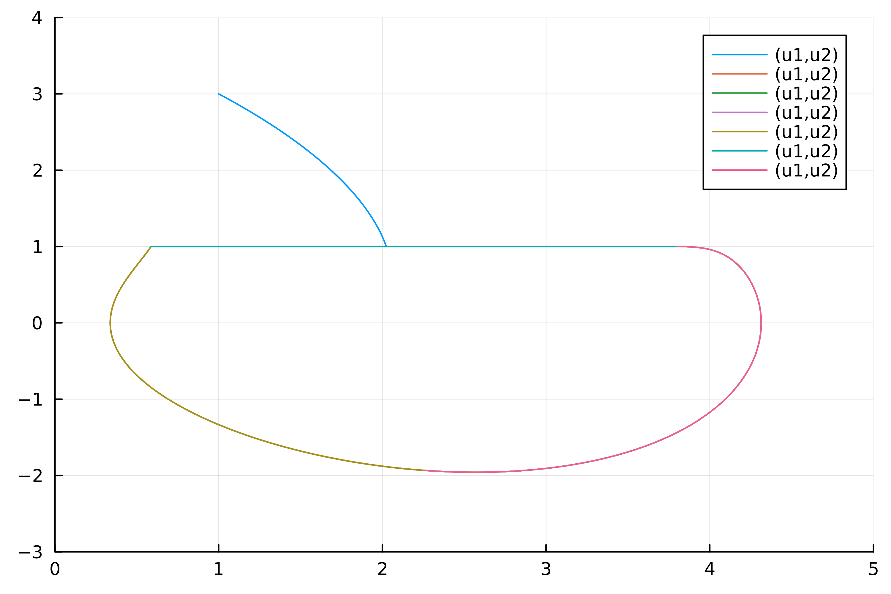
这个博客是由这个帖子扩展得到的.

参考文献

L. Dieci and L. Lopez.Fundamental matrix solutions of piecewise smooth differential systems. Mathematics and Computers in Simulation, 81(5):932–953, 2011.

Website built with Franklin.jl and Julia.