非光滑一维流形

或许这个软件包最值得注意的地方就是其可以计算非光滑流形. 目前, 支持两类系统的非光滑流形计算:

• 时间周期的非光滑微分方程的一维流形计算
• 非光滑自治系统的二维流形计算

其中流形值得都是鞍点的不变流形, 前者需要取时间周期映射, 后者则需要取固定步长的时间-$T$-映射. 这两类系统中的非光滑因素可以是多种多样的, 包括分段光滑, 碰撞, 以及它们之间的组合. 这三类非光滑系统无需用户自己求解, 我们提供了三个封装的结构体:

• PiecewiseV
• BilliardV
• PiecewiseImpactV

并使用 OrdinaryDiffEq.jl 中的 Callback 功能来进行时间映射的计算. 下面将以三个例子来介绍这三类非光滑系统不变流形的计算方法.

分段光滑系统

考虑一个简单的分段光滑系统:

\[\begin{aligned} \dot{x}&=y,\\ \dot{y}&=f(x) + \epsilon \sin(2\pi t), \end{aligned}\]

其中

\[f(x) = \begin{cases} -k_1 x& \text{if } x < -d,\\ k_2 x & \text{if } -d<x<d,\\ -k_3 x& \text{if } x > d. \end{cases}\]

\[k_1,k_2,k_3,d>0\]

都为正的常数. 下面我们将计算时间周期映射的不变流形. 注意到当周期扰动很小时, 鞍点应当很接近原点.

首先加载用到的程序包

julia> using InvariantManifolds, LinearAlgebra, StaticArrays, OrdinaryDiffEq, CairoMakie

接着定义分段光滑的矢量场:

f1(x, p, t) = SA[x[2], p[1]*x[1]+p[4]*sin(2pi * t)]
f2(x, p, t) = SA[x[2], -p[2]*x[1]+p[4]*sin(2pi * t)]
f3(x, p, t) = SA[x[2], -p[3]*x[1]+p[4]*sin(2pi * t)]

hyper1(x, p, t) = x[1] - p[5]
hyper2(x, p, t) = x[1] + p[5]

dom1(x, p, t) = -p[5] < x[1] < p[5]
dom2(x, p, t) = x[1] > p[5]
dom3(x, p, t) = x[1] < -p[5]

vectorfield = PiecewiseV((f1, f2, f3), (dom1, dom2, dom3), (hyper1, hyper2))

PiecewiseV: 
fs: (Main.f1, Main.f2, Main.f3)
regions: (Main.dom1, Main.dom2, Main.dom3)
hypers: (Main.hyper1, Main.hyper2)
n: 0

传递给 PiecewiseV 这个结构体的参数分别为: 矢量场, 它们所在的区域, 以及分割这些区域的超平面. 更多细节可参考 PiecewiseV.

接下来我们将求解时间周期映射的关键信息封装到另外一个结构体 NSSetUp 中:

julia> setup = setmap(vectorfield, (0.0, 1.0), Tsit5(), abstol=1e-8)NSSetUp:
f: PiecewiseV{Tuple{typeof(Main.f1), typeof(Main.f2), typeof(Main.f3)}, Tuple{typeof(Main.dom1), typeof(Main.dom2), typeof(Main.dom3)}, Tuple{typeof(Main.hyper1), typeof(Main.hyper2)}}((Main.f1, Main.f2, Main.f3), (Main.dom1, Main.dom2, Main.dom3), (Main.hyper1, Main.hyper2), 0)
timespan: (0.0, 1.0)

其中函数 setmap 用于封装时间映射的计算信息. 现在我们已经定义好求解时间周期映射的一切了.

接下来为了生成局部流形. 我们同样需要定位鞍点以及其不稳定特征向量. 取定参数:

julia> para = para = [2, 5, 5, 0.6, 2]5-element Vector{Float64}:
 2.0
 5.0
 5.0
 0.6
 2.0

由于扰动是很小的, 鞍型的周期轨道应该仍然在 dom1 中. 因此我们可以使用 findsaddle 来计算鞍点的位置:

function df1(x, p, t)
    SA[0 1; p[1] 0]
end
initialguess = SA[0.0, 0.0]
saddle = findsaddle(f1, df1, (0.0,1.0), initialguess, para, abstol=1e-10)

Saddle{2,Float64,Float64}: 
saddle: [1.3120846754625683e-11, -0.0908885006640104]
unstable_directions: StaticArraysCore.SVector{2, Float64}[[0.5773502691896258, 0.816496580927726]]
unstable_eigen_values: [4.113250379341709]

接下来创建问题, 生成局部流形, 并进行延拓

julia> prob = NSOneDManifoldProblem(setup, para, ϵ = 1e-3)NSOneDManifoldProblem:
f: NSSetUp generated by non-smooth vector field: PiecewiseV{Tuple{typeof(Main.f1), typeof(Main.f2), typeof(Main.f3)}, Tuple{typeof(Main.dom1), typeof(Main.dom2), typeof(Main.dom3)}, Tuple{typeof(Main.hyper1), typeof(Main.hyper2)}}((Main.f1, Main.f2, Main.f3), (Main.dom1, Main.dom2, Main.dom3), (Main.hyper1, Main.hyper2), 0)
para: [2.0, 5.0, 5.0, 0.6, 2.0]
amax: 0.5
d: 0.001
ϵ: 0.001
dsmin: 1.0e-6
julia> segment = gen_segment(saddle)50-element Vector{StaticArraysCore.SVector{2, Float64}}:
 [1.3120846754625683e-11, -0.0908885006640104]
 [0.00011782659866974998, -0.09072186870871903]
 [0.00023565318421865322, -0.09055523675342765]
 [0.0003534797697675564, -0.09038860479813628]
 [0.0004713063553164597, -0.0902219728428449]
 [0.000589132940865363, -0.09005534088755354]
 [0.0007069595264142661, -0.08988870893226217]
 [0.0008247861119631695, -0.0897220769769708]
 [0.0009426126975120726, -0.08955544502167942]
 [0.001060439283060976, -0.08938881306638805]
 ⋮
 [0.0048308900206258795, -0.08405659049706411]
 [0.004948716606174783, -0.08388995854177275]
 [0.005066543191723685, -0.08372332658648138]
 [0.005184369777272589, -0.08355669463119]
 [0.005302196362821493, -0.08339006267589863]
 [0.005420022948370395, -0.08322343072060726]
 [0.005537849533919299, -0.08305679876531588]
 [0.005655676119468201, -0.08289016681002451]
 [0.005773502705017105, -0.08272353485473313]
julia> manifold = growmanifold(prob, segment, 8)Non-smooth one-dimensional manifold
Curves number: 30
Points number: 158521
Total arc length: 91.63468743374115
Flaw points number: 11
Distance failed points number: 0
Curvature failed points number: 11
Max dα in Flaw Points: 1.2460760164693181e-6

注意到, manifold.data 的数据类型是 Vector{Vector{S}}, 其中 S 是插值函数. 所以绘制结果需要使用如下函数:

using CairoMakie
function manifold_plot(data)
    fig = Figure()
    axes = Axis(fig[1,1])
    for k in eachindex(data)
        for j in eachindex(data[k])
            points=data[k][j].u
            lines!(axes,first.(points),last.(points))
        end
    end
    fig
end
manifold_plot(manifold.data)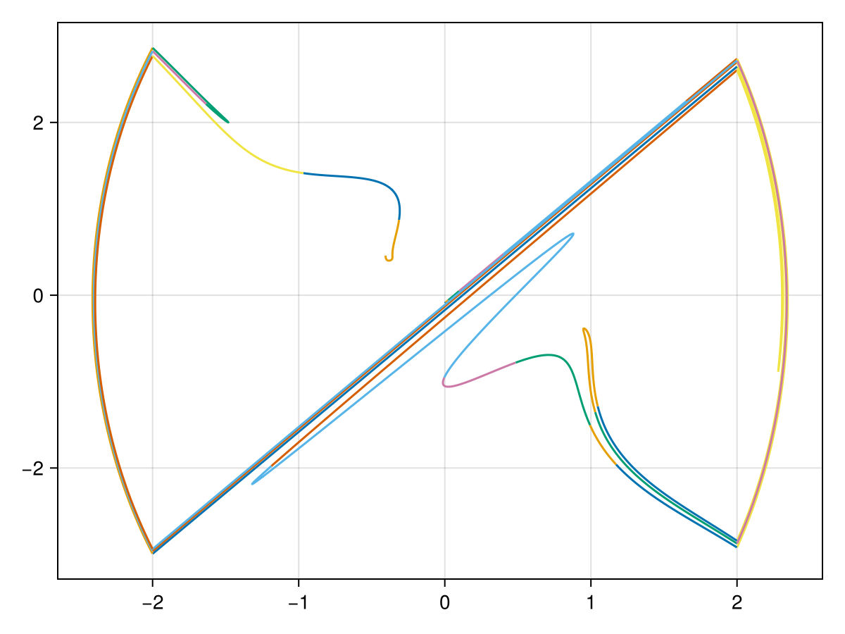

完整代码:

using InvariantManifolds, LinearAlgebra, StaticArrays, OrdinaryDiffEq, CairoMakie
f1(x, p, t) = SA[x[2], p[1]*x[1]+p[4]*sin(2pi * t)]
f2(x, p, t) = SA[x[2], -p[2]*x[1]+p[4]*sin(2pi * t)]
f3(x, p, t) = SA[x[2], -p[3]*x[1]+p[4]*sin(2pi * t)]
hyper1(x, p, t) = x[1] - p[5]
hyper2(x, p, t) = x[1] + p[5]
dom1(x, p, t) = -p[5] < x[1] < p[5]
dom2(x, p, t) = x[1] > p[5]
dom3(x, p, t) = x[1] < -p[5]
vectorfield = PiecewiseV((f1, f2, f3), (dom1, dom2, dom3), (hyper1, hyper2))
setup = setmap(vectorfield, (0.0, 1.0), Tsit5(), abstol=1e-8)
para = [2, 5, 5, 0.6, 2]
function df1(x, p, t)
    SA[0 1; p[1] 0]
end
initialguess = SA[0.0, 0.0]
saddle = findsaddle(f1, df1, (0.0,1.0), initialguess, para, abstol=1e-10)
prob = NSOneDManifoldProblem(setup, para, ϵ = 1e-3)
segment = gen_segment(saddle)
manifold = growmanifold(prob, segment, 8)
function manifold_plot(data)
    fig = Figure()
    axes = Axis(fig[1,1])
    for k in eachindex(data)
        for j in eachindex(data[k])
            points=data[k][j].u
            lines!(axes,first.(points),last.(points))
        end
    end
    fig
end
manifold_plot(manifold.data)

碰撞系统

考虑如下的受到激励的倒摆方程:

\[\begin{aligned} \dot{x}&= y,\\ \dot{y}&= \sin(x) - \epsilon \cos(2\pi t), \end{aligned}\]

假设倒摆两边存在墙壁: 当 $x=\xi$ 或者 $x=-\xi$ 时, 有 $y\rightarrow - ry$. 同样地, 需要先构建非光滑矢量场

f(x, p, t) = SA[x[2], sin(x[1])-p[1]*cos(2 * pi * t)]

hyper1(x, p, t) = x[1] + p[2]
hyper2(x, p, t) = x[1] - p[2]

rule1(x, p, t) = SA[x[1], -p[3]*x[2]]
rule2(x, p, t) = SA[x[1], -p[3]*x[2]]

vectorfield = BilliardV(f, (hyper1, hyper2), (rule1, rule2))

BilliardV{typeof(Main.f), Tuple{typeof(Main.hyper1), typeof(Main.hyper2)}, Tuple{typeof(Main.rule1), typeof(Main.rule2)}}(Main.f, (Main.hyper1, Main.hyper2), (Main.rule1, Main.rule2))

接着封装求解时间周期映射的信息:

setup = setmap(vectorfield, (0.0, 1.0), Vern9(), abstol=1e-10)

NSSetUp:
f: BilliardV{typeof(Main.f), Tuple{typeof(Main.hyper1), typeof(Main.hyper2)}, Tuple{typeof(Main.rule1), typeof(Main.rule2)}}(Main.f, (Main.hyper1, Main.hyper2), (Main.rule1, Main.rule2))
timespan: (0.0, 1.0)

寻找鞍点:

function df(x, p, t)
    SA[0 1; cos(x[1]) 0]
end
para = [0.2, pi / 4, 0.98]
initialguess = SA[0.0, 0.0]
saddle = findsaddle(f, df, (0.0,1.0), initialguess, para, abstol=1e-10)

Saddle{2,Float64,Float64}: 
saddle: [0.004940905039667357, 3.526850741022572e-11]
unstable_directions: StaticArraysCore.SVector{2, Float64}[[0.7071078867575611, 0.7071056756138056]]
unstable_eigen_values: [2.7182735331462027]

接下来创建问题, 生成局部流形, 并进行延拓

julia> prob = NSOneDManifoldProblem(setup, para)NSOneDManifoldProblem:
f: NSSetUp generated by non-smooth vector field: BilliardV{typeof(Main.f), Tuple{typeof(Main.hyper1), typeof(Main.hyper2)}, Tuple{typeof(Main.rule1), typeof(Main.rule2)}}(Main.f, (Main.hyper1, Main.hyper2), (Main.rule1, Main.rule2))
para: [0.2, 0.7853981633974483, 0.98]
amax: 0.5
d: 0.001
ϵ: 1.0e-5
dsmin: 1.0e-6
julia> segment = gen_segment(saddle)50-element Vector{StaticArraysCore.SVector{2, Float64}}:
 [0.004940905039667357, 3.526850741022572e-11]
 [0.005085212771658696, 0.00014430731600601876]
 [0.0052295205036500345, 0.0002886145967435301]
 [0.005373828235641373, 0.0004329218774810414]
 [0.005518135967632713, 0.0005772291582185528]
 [0.005662443699624052, 0.0007215364389560641]
 [0.005806751431615391, 0.0008658437196935754]
 [0.0059510591636067305, 0.001010151000431087]
 [0.006095366895598069, 0.0011544582811685983]
 [0.006239674627589408, 0.0012987655619061094]
 ⋮
 [0.010857522051312258, 0.005916598545506474]
 [0.011001829783303595, 0.006060905826243984]
 [0.011146137515294932, 0.006205213106981495]
 [0.011290445247286273, 0.006349520387719007]
 [0.011434752979277613, 0.006493827668456518]
 [0.01157906071126895, 0.006638134949194029]
 [0.011723368443260291, 0.006782442229931541]
 [0.011867676175251628, 0.006926749510669052]
 [0.012011983907242969, 0.007071056791406564]
julia> manifold = growmanifold(prob, segment, 11)Non-smooth one-dimensional manifold
Curves number: 38
Points number: 96016
Total arc length: 63.81546496506779
Flaw points number: 3
Distance failed points number: 0
Curvature failed points number: 3
Max dα in Flaw Points: 2.4211133374319635e-7

最后绘制结果:

manifold_plot(manifold.data)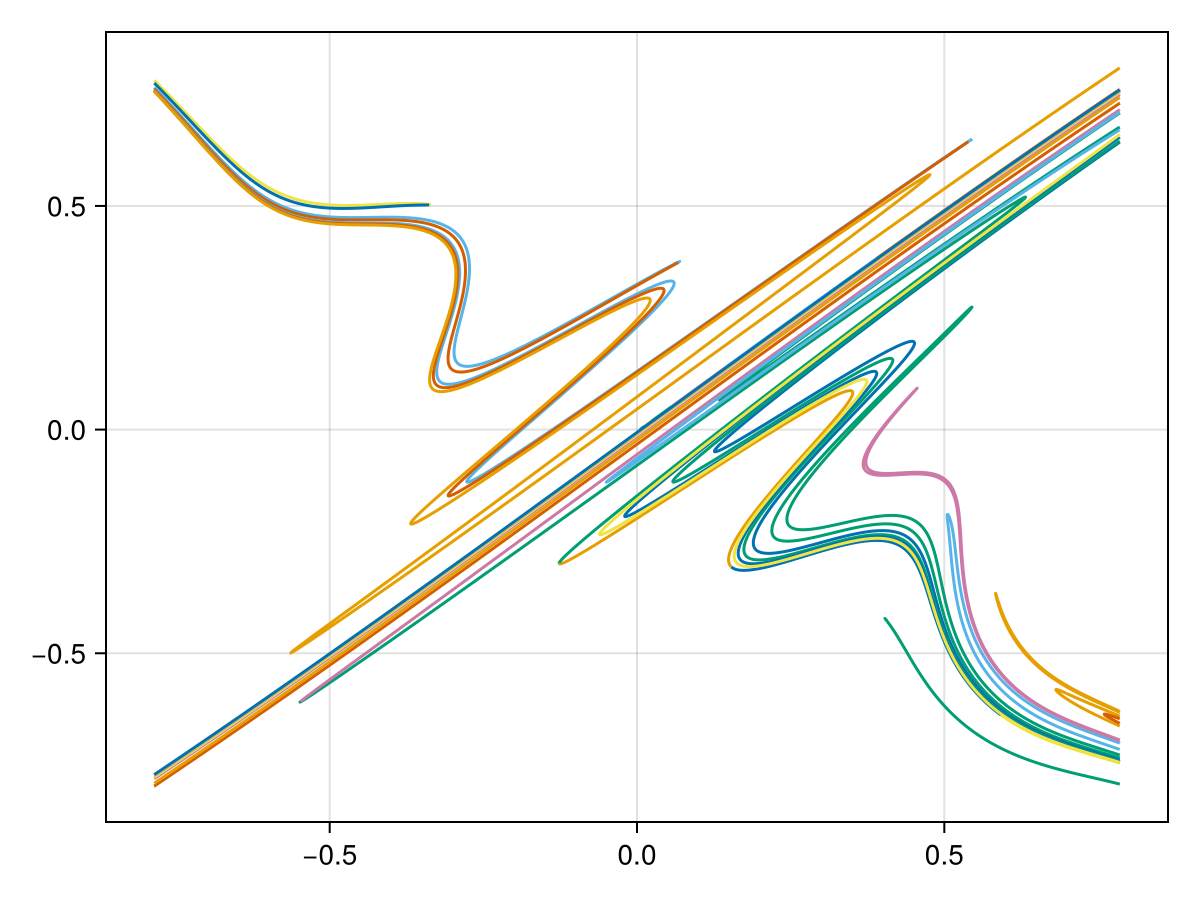

完整代码:

using InvariantManifolds, LinearAlgebra, StaticArrays, OrdinaryDiffEq, CairoMakie
f(x, p, t) = SA[x[2], sin(x[1])-p[1]*cos(2 * pi * t)]
hyper1(x, p, t) = x[1] + p[2]
hyper2(x, p, t) = x[1] - p[2]
rule1(x, p, t) = SA[x[1], -p[3]*x[2]]
rule2(x, p, t) = SA[x[1], -p[3]*x[2]]
vectorfield = BilliardV(f, (hyper1, hyper2), (rule1, rule2))
setup = setmap(vectorfield, (0.0, 1.0), Vern9(), abstol=1e-10)
function df(x, p, t)
    SA[0 1; cos(x[1]) 0]
end
para = [0.2, pi / 4, 0.98]
initialguess = SA[0.0, 0.0]
saddle = findsaddle(f, df, (0.0,1.0), initialguess, para, abstol=1e-10)
prob = NSOneDManifoldProblem(setup, para)
segment = gen_segment(saddle)
manifold = growmanifold(prob, segment, 11)
function manifold_plot(data)
    fig = Figure()
    axes = Axis(fig[1,1])
    for k in eachindex(data)
        for j in eachindex(data[k])
            points=data[k][j].u
            lines!(axes,first.(points),last.(points))
        end
    end
    fig
end
manifold_plot(manifold.data)

分段光滑与碰撞的组合的 ODE 系统

现在考虑同时存在分段光滑与碰撞的 ODE 系统:

\[\begin{aligned} \dot{x}&=y,\\ \dot{y}&=f(x) + \epsilon \sin(2\pi t), \end{aligned}\]

其中

\[f(x) = \begin{cases} -k_1 x& \text{if } x < -d,\\ k_2 x & \text{if } -d<x<d \end{cases}\]

\[k_1,k_2,d>0\]

都为正的常数. 当 $x=d$ 时, 有 $\dot{y}->-r\dot{y}$. 下面我们将计算时间周期映射的不变流形. 注意到当周期扰动很小时, 鞍点应当很接近原点. 首先加载用到的程序包

julia> using InvariantManifolds, LinearAlgebra, StaticArrays, OrdinaryDiffEq, CairoMakie

接着定义非光滑矢量场:

f1(x, p, t) = SA[x[2], p[1]*x[1]+p[3]*sin(2pi * t)]
f2(x, p, t) = SA[x[2], -p[2]*x[1]+p[3]*sin(2pi * t)]

hyper1(x, p, t) = x[1] - p[4]
hyper2(x, p, t) = x[1] + p[4]

dom1(x, p, t) = -p[4] < x[1]
dom2(x, p, t) = x[1] < -p[4]

impact_rule(x, p, t) = SA[x[1], -p[5]*x[2]]
id(x,p,t) = x

vectorfield = PiecewiseImpactV((f1, f2), (dom1, dom2), (hyper1, hyper2), (impact_rule, id), [1])

PiecewiseImpactV{Tuple{typeof(Main.f1), typeof(Main.f2)}, Tuple{typeof(Main.hyper1), typeof(Main.hyper2)}, Tuple{typeof(Main.impact_rule), typeof(Main.id)}, Tuple{typeof(Main.dom1), typeof(Main.dom2)}}((Main.f1, Main.f2), (Main.dom1, Main.dom2), (Main.hyper1, Main.hyper2), (Main.impact_rule, Main.id), [1], 0)

传递给 PiecewiseImpactV 这个结构体的参数分别为: 矢量场, 它们所在的区域, 以及分割这些区域的超平面, 作用在超平面上的规则, 以及具有碰撞效应的那些规则列表. 更多细节可参考 PiecewiseImpactV.

接下来我们将求解时间周期映射的关键信息封装到另外一个结构体 NSSetUp 中:

julia> setup = setmap(vectorfield, (0.0, 1.0), Tsit5(), abstol=1e-8, reltol=1e-8)NSSetUp:
f: PiecewiseImpactV{Tuple{typeof(Main.f1), typeof(Main.f2)}, Tuple{typeof(Main.hyper1), typeof(Main.hyper2)}, Tuple{typeof(Main.impact_rule), typeof(Main.id)}, Tuple{typeof(Main.dom1), typeof(Main.dom2)}}((Main.f1, Main.f2), (Main.dom1, Main.dom2), (Main.hyper1, Main.hyper2), (Main.impact_rule, Main.id), [1], 0)
timespan: (0.0, 1.0)

其中函数 setmap 用于封装时间映射的计算信息. 现在我们已经定义好求解时间周期映射的一切了.

接下来为了生成局部流形. 我们同样需要定位鞍点以及其不稳定特征向量. 取定参数:

julia> para = [2, 5, 0.5, 2, 0.98]5-element Vector{Float64}:
 2.0
 5.0
 0.5
 2.0
 0.98

由于扰动是很小的, 鞍型的周期轨道应该仍然在 dom1 中. 因此我们可以使用 findsaddle 来计算鞍点的位置:

function df1(x, p, t)
    SA[0 1; p[1] 0]
end
initialguess = SA[0.0, 0.0]
saddle = findsaddle(f1, df1, (0.0,1.0), initialguess, para, abstol=1e-10)

Saddle{2,Float64,Float64}: 
saddle: [7.410052858050141e-12, -0.0757404172152893]
unstable_directions: StaticArraysCore.SVector{2, Float64}[[0.5773502691896258, 0.816496580927726]]
unstable_eigen_values: [4.113250379341709]

接下来创建问题, 生成局部流形, 并进行延拓

julia> prob = NSOneDManifoldProblem(setup, para)NSOneDManifoldProblem:
f: NSSetUp generated by non-smooth vector field: PiecewiseImpactV{Tuple{typeof(Main.f1), typeof(Main.f2)}, Tuple{typeof(Main.hyper1), typeof(Main.hyper2)}, Tuple{typeof(Main.impact_rule), typeof(Main.id)}, Tuple{typeof(Main.dom1), typeof(Main.dom2)}}((Main.f1, Main.f2), (Main.dom1, Main.dom2), (Main.hyper1, Main.hyper2), (Main.impact_rule, Main.id), [1], 0)
para: [2.0, 5.0, 0.5, 2.0, 0.98]
amax: 0.5
d: 0.001
ϵ: 1.0e-5
dsmin: 1.0e-6
julia> segment = gen_segment(saddle)50-element Vector{StaticArraysCore.SVector{2, Float64}}:
 [7.410052858050141e-12, -0.0757404172152893]
 [0.0001178265929589561, -0.07557378525999793]
 [0.00023565317850785932, -0.07540715330470656]
 [0.00035347976405676254, -0.07524052134941518]
 [0.0004713063496056658, -0.07507388939412381]
 [0.000589132935154569, -0.07490725743883245]
 [0.0007069595207034722, -0.07474062548354107]
 [0.0008247861062523756, -0.0745739935282497]
 [0.0009426126918012787, -0.07440736157295832]
 [0.001060439277350182, -0.07424072961766695]
 ⋮
 [0.004830890014915086, -0.06890850704834302]
 [0.004948716600463989, -0.06874187509305166]
 [0.0050665431860128915, -0.06857524313776028]
 [0.005184369771561795, -0.06840861118246891]
 [0.005302196357110699, -0.06824197922717753]
 [0.0054200229426596015, -0.06807534727188616]
 [0.005537849528208505, -0.06790871531659479]
 [0.005655676113757407, -0.06774208336130341]
 [0.0057735026993063114, -0.06757545140601204]
julia> manifold = growmanifold(prob, segment, 9)Non-smooth one-dimensional manifold
Curves number: 52
Points number: 292201
Total arc length: 175.48287334895554
Flaw points number: 2
Distance failed points number: 0
Curvature failed points number: 2
Max dα in Flaw Points: 1.4116867284183935e-7

注意到, manifold.data 的数据类型是 Vector{Vector{S}}, 其中 S 是插值函数. 所以绘制结果需要使用如下函数:

using CairoMakie
function manifold_plot(data)
    fig = Figure()
    axes = Axis(fig[1,1])
    for k in eachindex(data)
        for j in eachindex(data[k])
            points=data[k][j].u
            lines!(axes,first.(points),last.(points))
        end
    end
    fig
end
manifold_plot(manifold.data)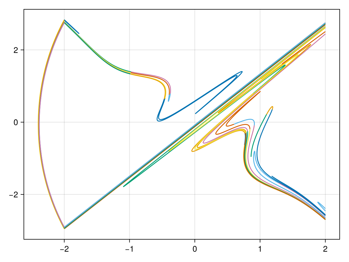

完整代码:

using InvariantManifolds, LinearAlgebra, StaticArrays, OrdinaryDiffEq, CairoMakie
f1(x, p, t) = SA[x[2], p[1]*x[1]+p[3]*sin(2pi * t)]
f2(x, p, t) = SA[x[2], -p[2]*x[1]+p[3]*sin(2pi * t)]
hyper1(x, p, t) = x[1] - p[4]
hyper2(x, p, t) = x[1] + p[4]
dom1(x, p, t) = -p[4] < x[1]
dom2(x, p, t) = x[1] < -p[4]
impact_rule(x, p, t) = SA[x[1], -p[5]*x[2]]
id(x,p,t) = x
vectorfield = PiecewiseImpactV((f1, f2), (dom1, dom2), (hyper1, hyper2), (impact_rule, id), [1])
setup = setmap(vectorfield, (0.0, 1.0), Tsit5(), abstol=1e-8, reltol=1e-8)
para = [2, 5, 0.5, 2, 0.98]
initialguess = SA[0.0, 0.0]
function df1(x, p, t)
    SA[0 1; p[1] 0]
end
saddle = findsaddle(f1, df1, (0.0,1.0), initialguess, para, abstol=1e-10)
segment = gen_segment(saddle)
prob = NSOneDManifoldProblem(setup, para)
manifold = growmanifold(prob, segment, 9)
function manifold_plot(data)
    fig = Figure()
    axes = Axis(fig[1,1])
    for k in eachindex(data)
        for j in eachindex(data[k])
            points=data[k][j].u
            lines!(axes,first.(points),last.(points))
        end
    end
    fig
end
manifold_plot(manifold.data)