非光滑两维流形

下面我们将继续以 Lorenz 系统为例, 不同的是我们将对这个系统引入一个人为的非光滑因素. 首先加载需要的包:

julia> using InvariantManifolds, LinearAlgebra, StaticArrays, OrdinaryDiffEq, CairoMakie, DataInterpolations

接着定义在远离原点时归一化的向量场:

julia> function lorenz(x, p, t)
           σ, ρ, β = p
           v = SA[σ*(x[2]-x[1]),
               ρ*x[1]-x[2]-x[1]*x[3],
               x[1]*x[2]-β*x[3]
           ]
           v / sqrt(0.1 + norm(v)^2)
       endlorenz (generic function with 1 method)

与先前的例子不同的是, 我们将引入如下非光滑因素: 当 $z=\xi$ 时, $(x,y,z)\rightarrow(x,-y,z)$. 因此, 我们需要定义一个带有碰撞因素的向量场:

hyper(x,p,t) = x[3]-p[4]
rule(x,p,t) = SA[x[1], -x[2], x[3]]
vectorfield =BilliardV(lorenz, (hyper,),(rule,))

BilliardV{typeof(Main.lorenz), Tuple{typeof(Main.hyper)}, Tuple{typeof(Main.rule)}}(Main.lorenz, (Main.hyper,), (Main.rule,))

接着如同前面的例子, 我们需要将求解这个微分方程的具体信息封装到 NSSetUp 中, 这需要使用函数 setmap:

julia> setup = setmap(vectorfield, (0.0, -1.0), Tsit5(), abstol=1e-8)NSSetUp:
f: BilliardV{typeof(Main.lorenz), Tuple{typeof(Main.hyper)}, Tuple{typeof(Main.rule)}}(Main.lorenz, (Main.hyper,), (Main.rule,))
timespan: (0.0, -1.0)

接着同样需要生成一个局部流形:

para = [10.0, 28.0, 8/3, 10.0]
function eigenv(p)
    σ, ρ, β = p
    [SA[0.0, 0.0, 1.0], SA[-(-1 + σ + sqrt(1 - 2 * σ + 4 * ρ * σ + σ^2))/(2*ρ), 1, 0]]
end
saddle = Saddle(SA[0, 0, 0.0], eigenv(para), [1.0, 1.0])
disk = gen_disk(saddle, r=1.0, d=0.1)

2-element Vector{Vector{StaticArraysCore.SVector{3, Float64}}}:
 [[0.0, 0.0, 0.0], [0.0, 0.0, 0.0], [0.0, 0.0, 0.0]]
 [[0.0, 0.0, 1.0], [-0.02591854368552384, 0.033247591065479865, 0.9991110182465031], [-0.05179100514622039, 0.06643606912734985, 0.9964456535631284], [-0.07757138408977644, 0.09950642628276328, 0.9920086448710159], [-0.10321384394323385, 0.1323998646435346, 0.9858078810097003], [-0.12867279334874365, 0.16505790087663877, 0.9778543867110426], [-0.1539029672233364, 0.19742247018544326, 0.9681623029976588], [-0.17885950723858804, 0.2294360295467975, 0.956748862040698], [-0.20349804157709053, 0.261041660020428, 0.9436343565216709], [-0.22777476382392425, 0.292183167948737, 0.9288421035528028]  …  [0.2277747638239243, -0.2921831679487371, 0.9288421035528028], [0.20349804157709064, -0.2610416600204281, 0.9436343565216709], [0.17885950723858818, -0.2294360295467977, 0.9567488620406979], [0.1539029672233366, -0.19742247018544354, 0.9681623029976587], [0.12867279334874349, -0.16505790087663855, 0.9778543867110426], [0.1032138439432337, -0.1323998646435344, 0.9858078810097004], [0.07757138408977632, -0.09950642628276313, 0.9920086448710159], [0.051791005146220315, -0.06643606912734974, 0.9964456535631284], [0.025918543685523803, -0.033247591065479816, 0.9991110182465031], [0.0, 0.0, 1.0]]

接着创建问题:

julia> prob = NSVTwoDManifoldProblem(setup, para, amax=0.5, d=0.5, ϵ=0.2, dsmin=1e-3)NSVTwoDManifoldProblem:
f: NSSetUp generated by non-smooth vector field: BilliardV{typeof(Main.lorenz), Tuple{typeof(Main.hyper)}, Tuple{typeof(Main.rule)}}(Main.lorenz, (Main.hyper,), (Main.rule,))
para: [10.0, 28.0, 2.6666666666666665, 10.0]
amax: 0.5
d: 0.5
ϵ: 0.2
dsmin: 0.001

最后计算流形, 并绘制图像:

manifold = growmanifold(prob, disk, 90, interp=LinearInterpolation)
function manifold_plot(annulus)
    fig = Figure()
    axes = LScene(fig[1, 1], show_axis=false, scenekw=(backgroundcolor=:white, clear=true))
    second(x) = x[2]
    for i in eachindex(annulus)
        for j in eachindex(annulus[i])
            points = annulus[i][j].u
            lines!(axes, first.(points), second.(points), last.(points), fxaa=true)
        end
    end
    fig
end
manifold_plot(manifold.data)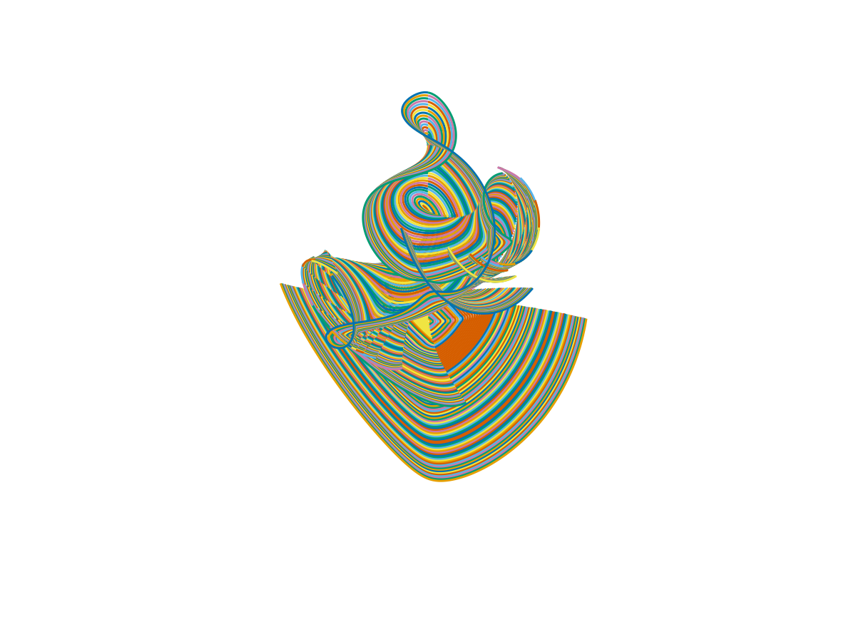

完整代码:

using InvariantManifolds, LinearAlgebra, StaticArrays, OrdinaryDiffEq, CairoMakie, DataInterpolations
function lorenz(x, p, t)
    σ, ρ, β = p
    v = SA[σ*(x[2]-x[1]),
        ρ*x[1]-x[2]-x[1]*x[3],
        x[1]*x[2]-β*x[3]
    ]
    v / sqrt(0.1 + norm(v)^2)
end
hyper(x,p,t) = x[3]-p[4]
rule(x,p,t) = SA[x[1], -x[2], x[3]]
vectorfield =BilliardV(lorenz, (hyper,),(rule,))
setup = setmap(vectorfield, (0.0, -1.0), Tsit5(), abstol=1e-8)
para = [10.0, 28.0, 8/3, 10.0]
function eigenv(p)
    σ, ρ, β = p
    [SA[0.0, 0.0, 1.0], SA[-(-1 + σ + sqrt(1 - 2 * σ + 4 * ρ * σ + σ^2))/(2*ρ), 1, 0]]
end
saddle = Saddle(SA[0, 0, 0.0], eigenv(para), [1.0, 1.0])
disk = gen_disk(saddle, r=1.0, d=0.1)
prob = NSVTwoDManifoldProblem(setup, para, amax=0.5, d=0.5, ϵ=0.2, dsmin=1e-3)
manifold = growmanifold(prob, disk, 90, interp=LinearInterpolation)
function manifold_plot(annulus)
    fig = Figure()
    axes = LScene(fig[1, 1], show_axis=false, scenekw=(backgroundcolor=:white, clear=true))
    second(x) = x[2]
    for i in eachindex(annulus)
        for j in eachindex(annulus[i])
            points = annulus[i][j].u
            lines!(axes, first.(points), second.(points), last.(points), fxaa=true)
        end
    end
    fig
end
manifold_plot(manifold.data)