光滑两维流形

在本质上, 我们并没有引入新的算法, 计算二维流形的核心函数跟一维流形的核心函数是一样的. 我们只是将二维流形表示为离得足够近的一维的圆圈.

自治向量场: Lorenz 流形

首先加载需要的包, 并定义 Lorenz 向量场:

julia> using InvariantManifolds, LinearAlgebra, StaticArrays, OrdinaryDiffEq, CairoMakie
julia> function lorenz(x, p, t)
           σ, ρ, β = p
           v = SA[σ*(x[2]-x[1]),
               ρ*x[1]-x[2]-x[1]*x[3],
               x[1]*x[2]-β*x[3]
           ]
           v / sqrt(0.1 + norm(v)^2)
       endlorenz (generic function with 1 method)

值得注意的是, 我们对向量场进行了一个近似的归一化, 使得向量场的模长保持在一个很小的范围内. 这样可以保证流形的扩张是均匀的. 在经典参数下:

julia> para = [10.0, 28.0, 8/3]3-element Vector{Float64}:
 10.0
 28.0
  2.6666666666666665

原点这个平衡点的 Jacobi 矩阵具有两个稳定方向, 这个稳定方向分别是:

function eigenv(p)
    σ, ρ, β = p
    [SA[0.0, 0.0, 1.0], SA[-(-1 + σ + sqrt(1 - 2 * σ + 4 * ρ * σ + σ^2))/(2*ρ), 1, 0]]
end
eigenv(para)

2-element Vector{StaticArraysCore.SVector{3, Float64}}:
 [0.0, 0.0, 1.0]
 [-0.7795615518272664, 1.0, 0.0]

那么我们可以创建一个 Saddle 结构体来存储这个鞍点:

julia> saddle = Saddle(SA[0, 0, 0.0], eigenv(para), [1.0, 1.0])Saddle{3,Float64,Float64}:
saddle: [0.0, 0.0, 0.0]
unstable_directions: StaticArraysCore.SVector{3, Float64}[[0.0, 0.0, 1.0], [-0.7795615518272664, 1.0, 0.0]]
unstable_eigen_values: [1.0, 1.0]

这里特征值的大小可以随意指定, 不会影响计算结果. 由于计算的是稳定流形, 我们需要将流进行反向演化. 定义如下映射:

julia> function lorenz_map(x, p)
           prob = ODEProblem{false}(lorenz, x, (0.0, -1.0), p)
           sol = solve(prob, Vern9(), abstol = 1e-10)
           sol[end]
       endlorenz_map (generic function with 1 method)

现在我们可以创建问题:

julia> prob = VTwoDManifoldProblem(lorenz_map, para, d=1.0, amax=1.0, dsmin=1e-3)VTwoDManifoldProblem:
f:Main.lorenz_map
para: [10.0, 28.0, 2.6666666666666665]
amax: 1.0
d: 1.0
dsmin: 0.001

这些关键字参数的含义可参考 VTwoDManifoldProblem.

与一维流形类似, 同样需要一个局部流形才能进行延拓. 相应的创建局部流形的函数为 gen_disk:

julia> disk = gen_disk(saddle, r=1.0)2-element Vector{Vector{StaticArraysCore.SVector{3, Float64}}}:
 [[0.0, 0.0, 0.0], [0.0, 0.0, 0.0], [0.0, 0.0, 0.0]]
 [[0.0, 0.0, 1.0], [-0.00010127432293440568, 0.00012991190073063764, 0.9999999864332046], [-0.00020254864312087533, 0.00025982379793629897, 0.9999999457328191], [-0.00030382295781147296, 0.0003897356880920077, 0.9999998778988444], [-0.00040509726425826294, 0.0005196475676727878, 0.9999997829312824], [-0.0005063715597133095, 0.0006495594331536636, 0.9999996608301356], [-0.0006076458414286776, 0.0007794712810096597, 0.9999995115954075], [-0.000708920106656432, 0.000909383107715801, 0.9999993352271019], [-0.0008101943526486386, 0.0010392949097471134, 0.9999991317252238], [-0.0009114685766573632, 0.001169206683578623, 0.9999989010897786]  …  [0.0009114685766575245, -0.0011692066835788302, 0.9999989010897786], [0.0008101943526485436, -0.0010392949097469916, 0.9999991317252238], [0.0007089201066560809, -0.0009093831077153506, 0.9999993352271019], [0.000607645841428499, -0.0007794712810094307, 0.9999995115954075], [0.0005063715597133038, -0.0006495594331536562, 0.9999996608301356], [0.0004050972642584299, -0.000519647567673002, 0.9999997829312824], [0.0003038229578118127, -0.0003897356880924434, 0.9999998778988444], [0.00020254864312095882, -0.00025982379793640603, 0.9999999457328191], [0.00010127432293423296, -0.0001299119007304161, 0.9999999864332046], [0.0, 0.0, 1.0]]

关于函数 gen_disk 的详细介绍请参考 gen_disk. 现在我们可以进行延拓了:

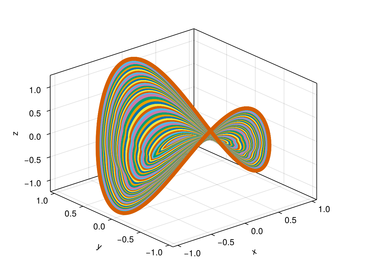
julia> manifold = growmanifold(prob, disk, 200)Two-dimensional manifold
Circles number: 202
Points number: 8028260
Flaw points number: 0

我们同样可以定义一个绘图函数来进行绘制结果:

using CairoMakie
function manifold_plot(annulus)
    fig = Figure()
    axes = LScene(fig[1, 1], show_axis=false, scenekw=(backgroundcolor=:white, clear=true))
    second(x) = x[2]
    for i in eachindex(annulus)
        points = annulus[i].u
        lines!(axes, first.(points), second.(points), last.(points), fxaa=true)
    end
    fig
end
manifold_plot(manifold.data)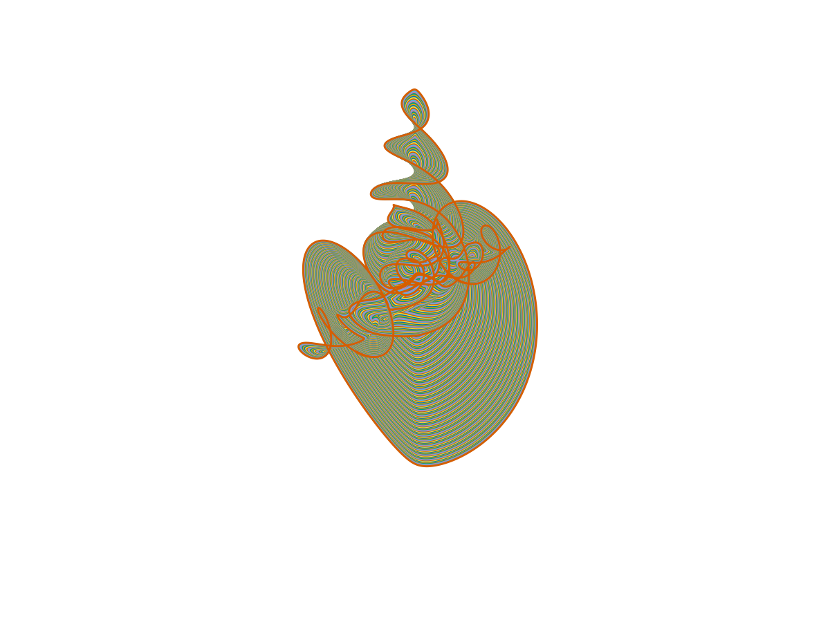

完整代码:

using InvariantManifolds, LinearAlgebra, StaticArrays, OrdinaryDiffEq, CairoMakie
function lorenz(x, p, t)
    σ, ρ, β = p
    v = SA[σ*(x[2]-x[1]),
        ρ*x[1]-x[2]-x[1]*x[3],
        x[1]*x[2]-β*x[3]
    ]
    v / sqrt(0.1 + norm(v)^2)
end
function eigenv(p)
    σ, ρ, β = p
    [SA[0.0, 0.0, 1.0], SA[-(-1 + σ + sqrt(1 - 2 * σ + 4 * ρ * σ + σ^2))/(2*ρ), 1, 0]]
end
para = [10.0, 28.0, 8/3]
saddle = Saddle(SA[0.0, 0.0, 0.0], eigenv(para), [1.0, 1.0])
prob = VTwoDManifoldProblem(lorenz, para, d=1.0, amax=1.0, dsmin=1e-3)
disk = gen_disk(saddle, r=1.0)
manifold = growmanifold(prob, disk, 200)
function manifold_plot(annulus)
    fig = Figure()
    axes = LScene(fig[1, 1], show_axis=false, scenekw=(backgroundcolor=:white, clear=true))
    second(x) = x[2]
    for i in eachindex(annulus)
        points = annulus[i].u
        lines!(axes, first.(points), second.(points), last.(points), fxaa=true)
    end
    fig
end
manifold_plot(manifold.data)

非线性映射

考虑如下的非线性映射:

\[f(X)=\varphi\circ\Lambda\circ\varphi^{-1}(X)\]

其中 $\varphi(x,y,z)=(x,y,z-\alpha x^2-\beta y^2)$ 是一个非线性映射, $\Lambda$ 是一个对角矩阵, 其对角元可用来控制映射 $f$ 在原点附近的 Jacobi 矩阵. 我们直接给出计算其不变流形的代码:

using InvariantManifolds, LinearAlgebra, StaticArrays, OrdinaryDiffEq, CairoMakie
const Λ = SDiagonal(SA[2.1, 6.3, 0.6])
φ(x, p)= SA[x[1],x[2],x[3]-p[1]*x[1]^2-p[2]*x[2]^2]
iφ(x, p)= SA[x[1],x[2],x[3]+p[1]*x[1]^2+p[2]*x[2]^2]
f(x,p) = φ(Λ*iφ(x, p),p)

para = [1.2,-1.2]
saddle = Saddle(SA[0.0, 0.0, 0.0], [SA[1.0, 0.0, 0.0], SA[0.0, 1.0, 0.0]], [2.1, 6.3])
prob = TwoDManifoldProblem(f, para, dcircle=0.05, d = 0.02, dsmin=1e-3)

disk = gen_disk(saddle, times=4, r= 0.05)
manifold = growmanifold(prob, disk, 3)
function manifold_plot(data)
    fig = Figure()
    axes = Axis3(fig[1,1])
    second(x) = x[2]
    for k in eachindex(data)
        for j in eachindex(data[k])
            points=data[k][j].u
            scatter!(axes,first.(points),second.(points),last.(points),fxaa=true)
        end
    end
    fig
end
manifold_plot(manifold.data)